Application and Advantages of Allegro's ATS344LSP Magnetically Back-Biased Differential Linear Sensor IC

Download PDF Version

By Yannick Vuillermet,
Allegro MicroSystems Europe Ltd.

Introduction

This application note aims to give insight on typical use of the Allegro ATS344LSP back-biased differential linear sensor IC. The main application of this sensor is to measure linear movements, such as shaft axial displacement.

For proper use, this sensor must be associated to a well designed moving ferromagnetic target. The back-bias arrangement and the differential sensing technique require a specific target shape to produce a useful magnetic signal.

The ATS344LSP includes a two-wire output interface and integrates a bypass capacitor into the package, which makes it suitable for decentralized sensing (typical in automotive applications) without the need for a printed circuit board.

The ATS344LSP offers unique performance benefits when compared to magnetic sensors generally used for linear position measurements.

In the following application note, the ATS344LSP sensing principle is described, advantages of its magnetic configuration are explained, and a typical user application is shown.

 

ATS344LSP Measurement Principle

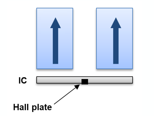
The ATS344LSP comprises, in a single package, two Hall plates, HP₁ and HP₂, separated by 3 mm, and a rare-earth magnet, positioned behind these sensing elements (see Figure 1).

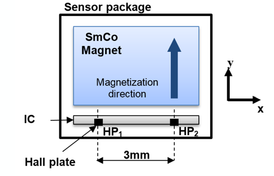
The magnet is magnetized along the y axis and both Hall plates measure the field strength along the y axis. The sensor measures the differential field ΔB = B₂ – B₁. B₂ is the field measured by HP₂ and B₁ is the field measured by HP₁.

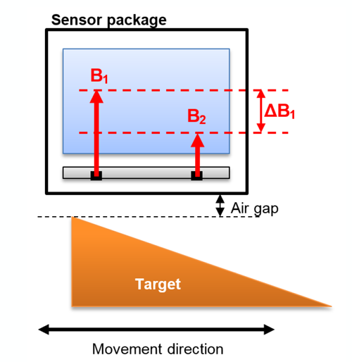
In Figure 2, the ATS344LSP sensor is placed in front of a basic ferromagnetic target. As a reminder, a ferromagnetic material is a material that gets magnetized when placed in an external magnetic field. Ferromagnetic materials also tend to concentrate local magnetic field lines. Most steels are ferromagnetic.

In this case, the target acquires a magnetization as a result of the sensor back-bias magnet. This target magnetization generates its own magnetic field, which is sensed by both Hall plates HP₁ and HP₂.

Both Hall plates also see background magnetic field from the magnet (called the magnet baseline). However, in an ideal case, the magnet baseline field is advantageously subtracted during the differential operation.

Because of the target shape in Figure 2, Hall plate 1 senses
more field than Hall plate 2: the differential field ΔB₁ = B₂ – B₁ is then negative and large.

In the following, air gap is defined as the distance between the closest point of the target to the sensor and the face of the sensor package (cf. Figure 2).

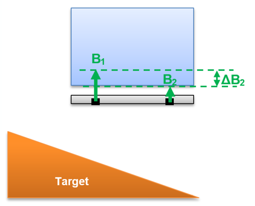
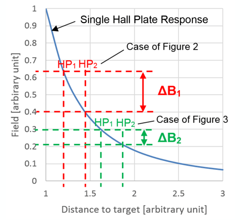
When the target is moved to the left, as in Figure 3, the differential field ΔB₂ is still negative but the difference is much smaller between B₁ and B₂. The reason for this change in differential magnetic field is the nonlinear behavior between the measured magnetic field level on a single Hall plate and the distance of the sensor to the target.

This nonlinear function can be seen in Figure 4, which demonstrates the typical behavior (with arbitrary units) of the field sensed by a single Hall plate versus the distance between this Hall plate and a ferromagnetic target. This figure also gives in red the case of Figure 2 and in green the case of Figure 3.

Consequently, the differential field ΔB sensed by the ATS344LSP is a direct measure of the unique position of the target (Figure 5).

 

Advantages of the ATS344LSP versus Other Magnetic Arrangements

The ATS344LSP offers a unique and advantageous method for measuring linear displacement. Other common techniques for measuring linear displacement are described below.

The first common technique uses a single field measurement (for example, a single Hall plate) in association with a zero-gauss (or 0 G) ring magnet (Figure 6). The zero-gauss magnet is a magnet
designed to have no field at the Hall plate position (i.e. magnet baseline is zero). The ring magnet is also magnetized along the y axis.

Zero-gauss magnets are used with single Hall plate ICs to limit the inaccuracy of the sensor that results from temperature variation (for example, a SmCo rare-earth magnet loses around 4% of
its strength at 150°C compared to 20°C). A non-zero-gauss magnet would have a high baseline magnetic field, and the variation of this field over temperature is difficult to compensate.

A corresponding Allegro IC for these types of linear displacement measurements would be, for example, the ATS341LSE.

The field sensed by the Hall plate of such zero-gauss systems is a nonlinear measurement of the distance between the sensor and the moving ferromagnetic target: the closer the target, the stronger
the field. The sensor response is demonstrated in Figure 4.

The main advantage of the 0 G arrangement is the simplicity of the concept. The drawbacks are mainly the expensive 0 G magnet (compared to a rectangular magnet) and the sensitivity to external
perturbing magnetic fields—any external field perturbation will be directly sensed by the single Hall plate. Note that it is also usually necessary to calibrate this type of sensor in the application to compensate for variations in the actual mounting air gap.

The second common technique for measuring linear displacement uses a permanent magnet mounted on the moving object to be sensed and a sensor which is able to measure the angle of the
magnetic field generated by this magnet.

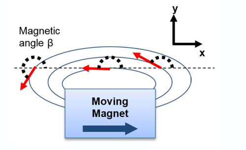
Figure 7 illustrates this principle: a moving magnet is magnetized along the x axis. The magnetic field angle β is measured and is a direct measurement of the magnet position.

Much more information on this principle can be found in the Allegro application note: “Linear Position Sensing Using Angle Sensor ICs” available on Allegro’s website. A corresponding Allegro IC for these types of linear displacement measurements would be, for example, the A1335.

The configuration in Figure 7 has a low sensitivity to air gap variations and, depending on the magnet design, is the only technique described in this application note that is able to reach large
air gaps (>4 mm) and long travel distances (>10 mm).

The main drawback of such a configuration is the need to mount the magnet on the moving object to be sensed in the system. The process of mounting the magnet is expensive, and there is always
the potential for the magnet to become displaced from the object.

In addition, the magnetic angle measurement is sensitive to external perturbing magnetic fields.

Because of the differential sensing principle used in the ATS344LSP, this IC is mostly insensitive to external magnetic field perturbation. A similar perturbation on both Hall plates (i.e. a common-mode field) is naturally rejected by the differential processing circuits used in the IC. The ATS344LSP remains sensitive to perturbations which are different on both Hall plates. For example, a wire parallel to the SP package leads, 40 mm away from the sensor and carrying 500 A, will generate a 2 G differential response that will be observed on the sensor output. But note that in this case, a single or a 2D field measurement would sense a 25 G variation.

The differential measurement technique of the ATS344LSP also allows for the use of a simple and cost-effective rectangular magnet instead of a complex and expensive zero-gauss magnet. Use of a simpler magnet is possible because the magnet baseline is canceled by the differential calculation in the ATS344LSP.

The use of a ferromagnetic target and an IC with an integrated back-bias magnet has many advantages, and there are also tradeoffs which must be considered. The main tradeoffs relate to the
operating air gap capability and the linear displacement sensing range of the IC. These parameters are limited by the size of the integrated magnet in Allegro SP package. For the SP package,
the typical maximum air gap is around 2 mm and the maximum sensed travel range is around 10 mm. In the case of a moving magnet technique, air gap capability and travel range can be much larger—at the cost of a very large and expensive magnet and reduced immunity to external perturbing fields.

In some applications, the moving object to be sensed is a shaft that will be linearly displaced but may also rotate around its axis. In this case, the moving magnet approach requires a magnet that
covers the full circumference of the shaft. This would also lead to an excessively large and expensive magnet.

As already discussed, the use of the ATS344LSP and a steel target to measure linear displacement is often much easier and less expensive when compared to mounting a discrete magnet.

Table 1: Comparison of Different Application Architectures for Linear Displacement Measurements

	0 G back bias and single measurement (ATS341LSE)	Moving magnet and magnetic field angle measurement (A1335)	ATS344LSP back-biased differential measurement
Max air gap [mm]	≈2	>4*	≈2
Typical stroke length [mm]	≈10	Depends on moving magnet Up to tens of mm*	≈10
Typical accuracy	Medium	High*	Medium
Calibration inside application	Recommended	Can be avoided	Recommended
Immunity to external perturbing field	Low	Low	High
Magnet	Integrated Complex shape	Depends on application	Integrated Simple shape
Target	Ferromagnetic	Permanent magnet	Ferromagnetic
Target mounting	Easy	Difficult	Easy

 
* Having good air gap capability, long range, and/or good accuracy is always at the cost of a large and expensive moving magnet.

Data in Table 1 are typical values only. For more details regarding a specific application, contact a local Allegro engineer.

Typical Application Example

Note that all results below are derived from simulations, and may differ slightly from real world results.

In this example, the goal is to determine the position of a target (Figure 8). The target moves along the x axis.

 

To illustrate the performances of the ATS344LSP sensor, consider a typical application with the requirements below:

• Static air gap: 1.35 ±0.45 mm
• Dynamic air gap: ±0.05 mm
• Temperature range: –40 to 150°C
• Travel range R: 10 mm
• 2 point calibration is conducted by the user at the end points of the linear stroke: 10/90% PWM output expected at these positions

To have a proper input field range, a V-shaped target is used, which generates a bipolar differential field on the ATS344LSP sensor.

As indicated previously, the magnetic field does not decrease linearly with the applications air gap (Figure 4). Consequently, using a straight V-shape target (Figure 9) will intrinsically lead to
a nonlinear differential sensor output and to accuracy error. This error is called the target intrinsic nonlinearity.

However, target shape optimizations could compensate for this intrinsic nonlinearity. Indeed, the field tends to decrease very quickly at close air gaps and much more slowly at large air gaps. Therefore, a target having a larger slope in the middle of the V-shape (i.e. where the Hall plates actually sense a large air gap) could compensate for the nonlinear magnetic field behavior.

A proper target design must also account for other application parameters (dynamic air gap variation, for example) and the sensor IC errors (offset drift with temperature, sensitivity drift with
temperature, etc.).

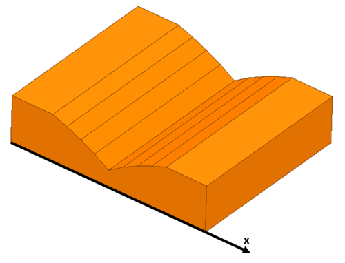
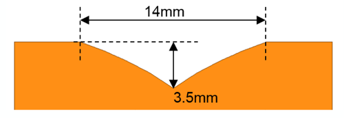
Figure 10 shows a cross-sectional view of the optimum target for the application example. A target length L of 14 mm has been chosen to not only fit the travel range and the distance between
both Hall plates (3 mm) but to also have margin regarding the V-shape end points. This margin is needed to avoid erroneous measurements from the flat regions outside the V-shape area. A 1 mm margin has been taken here. The target length L is then given by:

L ≥ R + 4 mm

For the V-shape height, values between 2 and 4 mm are recommended (3.5 mm is shown in Figure 10). Heights smaller than 2 mm would lead to small differential fields and consequently to
higher position inaccuracy. A height larger than 4 mm would not increase the field substantially because the ferromagnetic material would be too far away from the sensor.

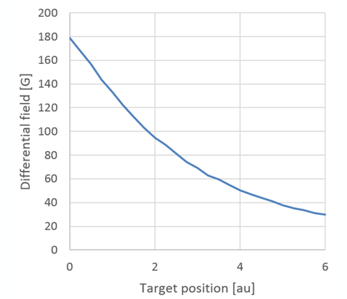
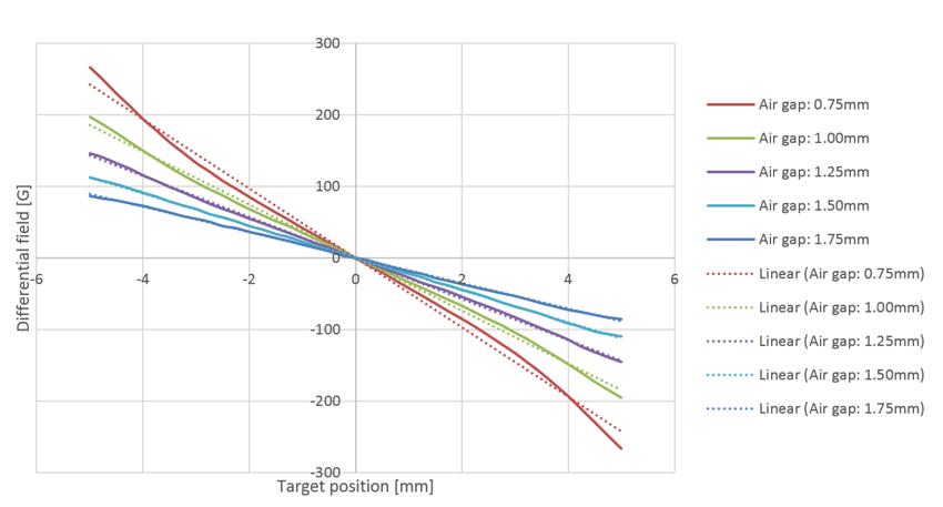
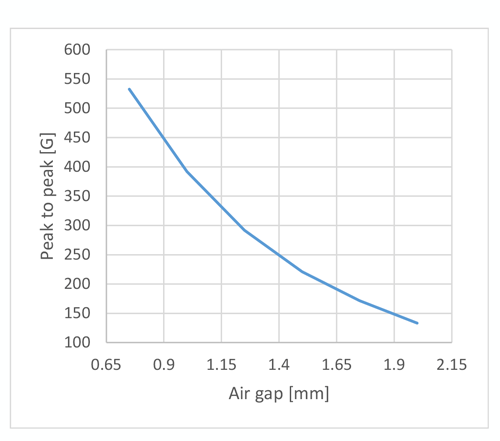
Figure 11 displays the differential field sensed by the ATS344LSP sensor in front of this optimum target versus target axial positionn and versus air gap. It can be seen that the differential field is linear at the nominal application air gap (1.35 mm) and at large air gaps, but deviates significantly at small air gaps. This is intentional: at small air gap the differential field sensed by the sensor is much higher (Figure 12) which makes the sensor much less sensitive to measurement errors (mainly IC offset drifts). Consequently, there is a compromise that must be made to obtain similar accuracy performance at small and large air gaps. At small air gaps, errors mostly come from intrinsic target nonlinearity, and at large air gaps, errors mostly come from sensor measurements errors.

Now, the accuracy expected for this application example will be evaluated. To obtain realistic values, a Monte Carlo statistical analysis was performed. In this simulation, thousands of realistic cases were modeled for varying application parameters (for example, mounting air gap and sensor offset error) according to their statistical distribution laws. For each of these cases, the sensor output accuracy was evaluated.

Results given are valid for the full IC temperature range and include sensor lifetime drift. The error reported here is the maximum position error for the full range of target displacement. The
offset drift over lifetime considered is ±12 G (based on the reduced temperature cycle testing that was performed on a similar product; this number will be confirmed by future testing on ATS344LSP).

The following mechanical distributions are assumed for performing the Monte Carlo analysis:

Parameter	Distribution	Mean [mm]	Standard deviation [mm]
Mounting Air Gap	Gaussian	1.35	0.15
Max Dynamic Air Gap	Gaussian; Only positive values are kept	0	0.05/3

 Figure 13 shows the distribution of the maximum position error over the full travel range for all the simulation cases evaluated. It includes mounting air gap, dynamic air gap variation, temperature variation, sensor errors, and target intrinsic nonlinearity. Sensor errors include offset and sensitivity drift with temperature, offset and sensitivity lifetime drift, sensor resolution and nonlinearity. Note that % FS (% Full Scale) stands for the percentage of the full linear travel range.

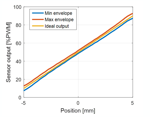
The sensor is calibrated, after mounting in the application, such that the first end of the travel range returns 10% PWM and second end returns 90% PWM (see Figure 14).

The average error is around 4.9% FS and the standard deviation is around 1.3% FS. From the error distribution analysis, it appears that around 3000 ppm of the samples have a maximum error
larger than 9.4% FS or 0.94 mm.

Although output linearization was not performed to compensate for intrinsic target nonlinearity, the final accuracy of the sensor is reasonably good.

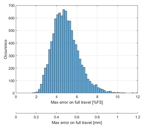
Figure 14 shows, for one random simulation case, the expected envelope of the sensor output with respect to all varied parameters.

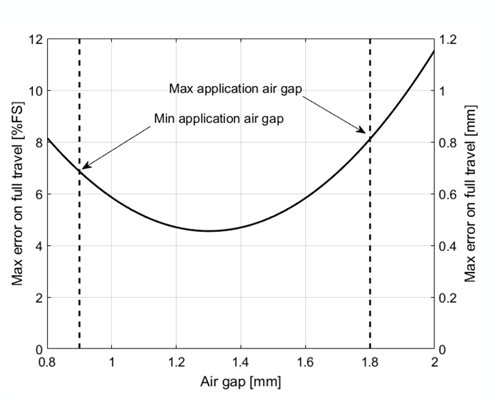
Figure 15 shows how the typical measurement error behaves versus the mounting air gap. As expected, the minimum error is around nominal air gap and the curve is approximately symmetric
relative to the mounting air gap range (0.9 to 1.8 mm).

 

Conclusions

Allegro Microsystems ATS344LSP magnetically back-biased differential linear sensor ICs offer unique advantages when measuring linear stroke position of a target or shaft. When compared to conventional zero-gauss back-biased linear ICs, or to magnetic angle sensor ICs sensing a moving magnet, the ATS344LSP offers:

• Elimination of magnets from the customer system
• Easy integration of a ferromagnetic target
• Very low sensitivity to external perturbing fields

Consequently, the ATS344LSP is recommended for use:

• in harsh magnetic environments,
• to simplify target mounting (cost reduction),
• to improve mechanical reliability of the target fixture in the application.

For more details on how ATS344LSP would perform in a specific application, contact a local Allegro application engineer.