Hall-Effect Sensors Applications Guide
Answering common sensor IC technology questions such as "What is Hall-effect?"
Allegro MicroSystems uses the latest integrated circuit technology in combination with the century-old Hall effect to produce Hall-effect sensor ICs. These are contactless, magnetically activated switches and sensor ICs with the potential to simplify and improve electrical and mechanical systems.
- Low-Cost Simplified Switching
- Efficient, Effective, Low-Cost Linear Sensor ICs
- Sensitive Circuits for Rugged Service
- Applications
- The Hall Effect: How Does It Work?
- Linear Output Hall-Effect Devices
- Digital Output Hall-Effect Switches
- Operation
- Characteristics and Tolerances
- Getting Started
- The Analysis
- Total Effective Air Gap (TEAG)
- Modes Of Operation
- Steep Slopes and High Flux Densities
- Vane Interruptor Switching
- Electrical Interface for Digital Hall Devices
- Common Interface Circuits
- Rotary Activators for Hall Switches
- Ring Magnets for Hall Switch Applications
- Bipolar Digital Switches
- Digital Latches
- Planar and Vertical Hall Devices
- Ring Magnets Detailed Discussion
- Temperature Effects
- An Inexpensive Alternative
- Ring Magnet Selection
- Ferrous Vane Rotary Activators
- A Ferrous Vane In Operation
- Rotor Design
- Material
- Vane/Window Widths, Rotor Size
- Steep Magnetic Slopes for Consistent Switching
- Small Air Gaps for Steep Slopes
- Flux Concentrators Pay Dividends
- Temperature Stability of Operate Point
- Calculating Dwell Angle and Duty Cycle Variations
- Effects of Bearing Wear
- Mounting also Affects Stability
- Quadrature
- Enhancement Considerations
- Individual Calibration Techniques
- Operating Modes: Head-On and Slide-By
- Operating Mode Enhancements:Compound Magnets
- Biased Operation
- Increasing Flux Density by Improving the Magnetic Circuit
- Flux Concentrators
- Feed-Throughs
- Magnet Selection
- Advanced Applications
- Current Limiting and Measuring Current Sensor ICs
- Multi-Turn Applications
- Other Applications for Linear Sensor ICs
- Using Calibrated Devices
- Glossary
Low-Cost Simplified Switching
Simplified switching is a Hall sensor IC strong point. Hall-effect IC switches combine Hall voltage generators, signal amplifiers, Schmitt trigger circuits, and transistor output circuits on a single integrated circuit chip. The output is clean, fast, and switched without bounce (an inherent problem with mechanical switches). A Hall-effect switch typically operates at up to a 100 kHz repetition rate, and costs less than many common electromechanical switches.
Efficient, Effective, Low-Cost Linear Hall-Effect Sensor ICs
The linear Hall-effect sensor IC detects the motion, position, or change in field strength of an electromagnet, a permanent magnet, or a ferromagnetic material with an applied magnetic bias. Energy consumption is very low. The output is linear and temperature-stable. The sensor IC frequency response is flat up to approximately 25 kHz.
A Hall-effect sensor IC is more efficient and effective than inductive or optoelectronic sensors, and at a lower cost.
topSensitive Circuits for Rugged Service
The Hall-effect sensor IC is virtually immune to environmental contaminants and is suitable for use under severe service conditions. The circuit is very sensitive and provides reliable, repetitive operation in close-tolerance applications.
Applications
Applications for Hall-effect ICs include use in ignition systems, speed controls, security systems, alignment controls, micrometers, mechanical limit switches, computers, printers, disk drives, keyboards, machine tools, key switches, and pushbutton switches. They are also used as tachometer pickups, current limit switches, position detectors, selector switches, current sensors, linear potentiometers, rotary encoders, and brushless DC motor commutators.
topWhat is Hall-effect?
The basic Hall element is a small sheet of semiconductor material, referred to as the Hall element, or active area, represented in figure 1.

Figure 1. Schematic representation of the active area of a Hall-effect device, with the Hall element represented by the component marked with an X
A constant voltage source, as shown in figure 2, forces a constant bias current, IBIAS , to flow in the semiconductor sheet. The output takes the form of a voltage, VHALL , measured across the width of the sheet. In the absence of a magnetic field, VHALL has a negligible value.

Figure 2. VHALL in the absence of a significant magnetic field
If the biased Hall element is placed in a magnetic field with flux lines at right angles to the bias current (see figure 3), the voltage output changes in direct proportion to the strength of the magnetic field. This is the Hall effect, discovered by E. F. Hall in 1879.

Figure 3. Hall effect, induced VHALL, resulting from significant magnetic flux (green arrows) perpendicular to the bias current flow
Linear Output Hall-Effect Devices
The output voltage of the basic Hall element is quite small. This can present problems, especially in an electrically noisy environment. Addition of a stable, high-quality DC amplifier and voltage regulator to the circuit (see figures 4 and 5) improves the transducer output and allows the device to operate over a wide range of supply voltages. The modified device provides an easy-to-use analog output that is linear and proportional to the applied magnetic flux density.

Figure 4. Hall circuit with amplification of VHALL

Figure 5. Hall device with voltage regulator and DC amplifier
For the most current list of linear output devices from Allegro, go to: Linear Position Sensor ICs.
topDigital Output Hall-Effect Switches
The addition of a Schmitt-trigger threshold detector with built-in hysteresis, as shown in figure 6, gives the Hall-effect circuit digital output capabilities. When the applied magnetic flux density exceeds a certain limit, the trigger provides a clean transition from off to on without contact bounce. Built-in hysteresis eliminates oscillation (spurious switching of the output) by introducing a magnetic dead zone in which switch action is disabled after the threshold value is passed.

Figure 6. Hall circuit with digital output capability
An open-collector NPN or N-channel FET (NFET) output transistor added to the circuit (see figure 7) gives the switch digital logic compatibility. The transistor is a saturated switch that shorts the output terminal to ground wherever the applied flux density is higher than the turn-on trip point of the device. The switch is compatible with all digital families. The output transistor can sink enough current to directly drive many loads, including relays, triacs, SCRs, LEDs, and lamps.

Figure 7. Common circuit elements for Hall switches
The circuit elements in figure 7, fabricated on a monolithic silicon chip and encapsulated in a small epoxy or ceramic package, are common to all Hall-effect digital switches. Differences between device types are generally found in specifications such as magnetic parameters, operating temperature ranges, and temperature coefficients.
topOperation
All Hall-effect devices are activated by a magnetic field. A mount for the devices and electrical connections must be provided. Parameters such as load current, environmental conditions, and supply voltage must fall within the specific limits shown in the datasheet.
Magnetic fields have two important characteristics: magnetic flux density, B (essentially, field strength), and magnetic field polarity (north or south). For Hall-devices, orientation of the field relative to the device active area also is important. The active area (Hall element) of Hall devices is embedded on a silicon chip located parallel to, and slightly inside of, one particular face of the package. That face is referred to as the branded face because it is normally the face that is marked with the part number (the datasheet for each device indicates the active area depth from the branded face). To optimally operate the switch, the magnetic flux lines must be oriented to cross perpendicularly through the active area (the branded face of planar Hall devices, or the sensitive edge of vertical Hall devices), and must have the correct polarity as it crosses through. Because the active area is closer to the branded face than it is to the back side of the case, and is exposed on the branded-face side of the chip, using this orientation produces a cleaner signal.
In the absence of any significant applied magnetic field, most Hall-effect digital switches are designed to be off (open circuit at output). They will turn on only if subjected to a magnetic field that has sufficient flux density and the correct polarity in the proper orientation. In switches, for example, if a south pole approaching the branded face would cause switching action, a north pole would have no effect. In practice, a close approach to the branded face of a planar Hall switch or along the sensitive edge of a vertical Hall switch by the south pole of a small permanent magnet (see figure 8) causes the output transistor to turn on. For a 3D Hall switch, the output(s) will turn on with a close approach of a magnet from any direction.

Figure 8. Operation of a Hall-effect device is activated by the motion of a magnet relative to the plane and centerline of the active area of the device
Transfer characteristic graphs can be used to plot this information. Figures 9 and 10 show output as a function of the magnetic flux density, B , (measured in gauss, G; 1 G = 0.1 mT) presented to the Hall element. The magnetic flux density is shown on the horizontal axis. The digital output of the Hall switch is shown along the vertical axis. Note that there is an algebraic convention applied, in which a strengthening south polarity field is indicated by an increasing positive B value, and a strengthening north polarity field is indicated by an increasing negative B value. For example, a +200 B field and a –200 B field are equally strong, but have opposite polarity (south and north, respectively).
As shown in figure 9, in the absence of an applied magnetic field (0 G), the switch is off, and the output voltage equals the power supply (12 V) due to the action of an external pull-up resistor. A permanent magnet south pole is then moved perpendicularly toward the active area of the device. As the magnet south pole approaches the branded face (for a planar Hall device) or the sensitive edge (for a vertical Hall device) of the switch, the Hall element is exposed to increasing positive magnetic flux density. At some point (240 G in this case), the output transistor turns on, and the output voltage approaches 0 V. That value of flux density is called the operate point, BOP. Continuing to increase the field strength has no effect; the switch has already turned on, and stays on. There is no upper limit to the magnetic field strength that may be applied to a Hall-effect sensor.

Figure 9. Transfer characteristics of a Hall switch being activated (switched on) by the increase in magnetic flux density from an approaching south pole
To turn the switch off, the magnetic flux density must fall to a value far lower than the 240 G operate point because of the built-in hysteresis of the device (these types of charts are sometimes referred to as hysteresis charts). For this example we use a 90 G hysteresis, which means the device turns off when the flux density decreases to 150 G (figure 10). That value of flux density is called the release point, BRP.

Figure 10. Transfer characteristics of a Hall switch being deactivated (switched off) by the decrease in magnetic flux density from an receding south pole
To acquire data for this graph, add a power supply and a pull-up resistor to limit current through the output transistor and enable the value of the output voltage to approach 0 V (see figure 11).

Figure 11. Test circuit for transfer characteristic charts
Characteristics and Tolerances
The exact magnetic flux density values required to turn Hall switches on and off differ for several reasons, including design criteria and manufacturing tolerances. Extremes in temperature will also somewhat affect the operate and release points, often referred to as the switching thresholds, or switchpoints.
For each device type, worst-case magnetic characteristics for the operate value, the release value, and hysteresis are provided in the datasheet.
All switches are guaranteed to turn on at or below the maximum operate point flux density. When the magnetic field is reduced, all devices will turn off before the flux density drops below the minimum release point value. Each device is guaranteed to have at least the minimum amount of hysteresis to ensure clean switching action. This hysteresis ensures that, even if mechanical vibration or electrical noise is present, the switch output is fast, clean, and occurs only once per threshold crossing.
topGetting Started
Because the electrical interface is usually straightforward, the design of a Hall-effect system should begin with the physical aspects. In position-sensing or motion-sensing applications, the following questions should be answered:
- How much and what type of motion is there?
- What angular or positional accuracy is required?
- How much space is available for mounting the sensing device and activating magnet?
- How much play is there in the moving assembly?
- How much mechanical wear can be expected over the lifetime of the machine?
- Will the product be a mass-produced assembly, or a limited number of machines that can be individually adjusted and calibrated?
- What temperature extremes are expected?
A careful analysis will pay big dividends in the long term.
topThe Analysis
The field strength of the magnet should be investigated. The strength of the field will be greatest at the pole face, and will decrease with increasing distance from the magnet. The strength of the magnetic field can be measured with a gaussmeter or a calibrated linear Hall sensor IC, and is a function of distance along the intended line of travel of the magnet. Hall device specifications (sensitivity in mV/G for a linear device, or operate and release points in gauss for a digital device) can be used to determine the critical distances for a particular magnet and type of motion. Note that these field strength plots are not linear, and that the shape of the flux density curve depends greatly upon magnet shape, the magnetic circuit, and the path traveled by the magnet.
topTotal Effective Air Gap (TEAG)
Total effective air gap (TEAG), is the sum of the active area depth (AAD, the depth of the Hall element below the branded face/edge of the device) and the air gap (AG, the distance between the package surface and the magnet or target surface). The AG is a mechanical clearance which should be as small as possible, consistent with dimensional tolerances of the magnet, bearing tolerances, bearing wear, and temperature effects on the Hall switch mounting bracket. Figure 12A is a graph of flux density as a function of TEAG, and illustrates the considerable increase in flux density at the sensor IC provided by a thinner package (the Allegro UA package has an AAD of about 0.50 mm). The actual gain depends predominantly on the characteristic slope of the flux density for the particular magnet used in the application. Note that the chart also shows the effect on flux density of other physical factors, such as package contribution from the device itself, and from any overmolding or protective covering of the sensor assembly in the application.
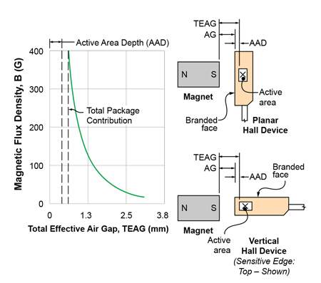
Figure 12A. Definition of total effective air gap, active area depth, and demonstration of the effects of the package itself on magnetic signal strength (for specifications of the magnet used for this data, see figure 25)
top
Modes Of Operation
Even with a simple bar or rod magnet, there are several possible paths for motion. The magnetic pole could move perpendicularly straight at the branded face of the planar Hall device, or the sensitive edge of the vertical Hall device. This is called the head-on mode of operation. The curve in figure 12B illustrates typical flux density (in gauss) as a function of TEAG for a cylindrical magnet.

Figure 12B. Demonstration of head-on mode of operation
The head-on mode is simple, works well, and is relatively insensitive to lateral motion. The designer should be aware that overextension of the mechanism could cause physical damage to the epoxy package of the Hall device if collision occurs.
A second configuration is moving the magnet from side to side across the Hall device, parallel to the branded face or the sensitive edge of the device package. This is referred to as the slide-by mode of operation, as illustrated in figure 13. Note that now the distance plotted on the horizontal axis of the chart is not total effective air gap, but rather the perpendicular distance from the centerline of the magnet to the centerline of the active area. Air gap is specified because of its obvious mechanical importance, but bear in mind that to do any calculations involving flux density, the package contribution must be added and the TEAG used, as before. The slide-by mode is commonly used to avoid contact if overextension of the mechanism is likely. The use of strong magnets and/or ferrous flux concentrators in well-designed slide-by magnetic circuits provides better sensing precision, with shorter travel of the magnet, than the head-on mode.

Figure 13. Demonstration of slide-by mode of operation, showing effect of changes in displacement between the centerlines of the magnet and the active area
Magnet manufacturers generally can provide head-on flux density curves for their magnets, but they often do not characterize them for slide-by operation, possibly because different air gap choices lead to an infinite number of these curves. However, after an air gap is chosen, the readily available head-on magnetic curves can be used to find the peak flux density (a single point) in the slide-by application by noting the value at the total effective air gap.
topSteep Slopes and High Flux Densities
For linear Hall devices, greater flux change for a given displacement gives greater output—clearly an advantage. The same property is desirable for digital Hall devices, but for more subtle reasons. To achieve consistent switching action in a given application, the Hall device must switch on and off at the same positions relative to the magnet.
To illustrate this concept, consider the flux density curves from two different magnet configurations, in figure 14. With an operate-point flux density of 200 G, a digital Hall-effect device would turn on at a distance of approximately 3.6 mm in either case. If manufacturing tolerances or temperature effects shifted the operate point to 300 G, notice that for curve A (steep slope) there is very little change in the distance at which switching occurs. In the case of curve B, the change is considerable. The release point (not shown) would be affected in much the same way. The basic principles illustrated in this example can be modified to include mechanism and device specification tolerances and can be used for worst-case design analysis. Examples of this procedure are shown in later sections.

Figure 14. Example of slide-by mode of operation, comparing the effects of two different Total Effective Air Gaps
top
Vane Interruptor Switching
In this mode, the activating magnet and the Hall device are mounted on a single rigid assembly with a small air gap between them. In this position, the Hall device is held in the On-state by the activating magnet. If a ferromagnetic plate, or vane, is placed between the magnet and the Hall device, as shown in figure 15, the vane forms a magnetic shunt that distorts the flux field away from the Hall device.

Figure 15. Demonstration of vane interruptor operation: (left) normal magnetic flux path without vane interruption, (right) vane shunting magnetic flux
Use of a movable vane is a practical way to switch a Hall device. The Hall device and magnet can be molded together as a unit, thereby eliminating alignment problems, to produce an extremely rugged switching assembly. The ferrous vane or vanes that interrupt the flux could have linear motion, or rotational motion, as in an automotive distributor. Ferrous vane assemblies, due to the steep flux density/ distance curves that can be achieved, are often used where precision switching over a large temperature range is required.
The ferrous vane can be made in many configurations, as shown in figure 16. With a linear vane similar to that of figure 16B, it is possible to repeatedly sense position within 0.05 mm over a 125°C temperature range.

Figure 16. Typical configurations for vane interruptors: (A) disk, (B), linear, and (C) cup
Electrical Interface for Digital Hall Devices
The output stage of a digital Hall switch is usually an open-collector NPN transistor (see figure 17). The rules for use are the same as those for any similar switching transistor. Certain digital Hall devices, particularly micropower devices, may have pushpull output stages constructed using MOSFET devices. These devices do not require an external pull-up resistor. Consult the device datasheet for details.
When the transistor is off, there is a small output leakage current (typically a few nanoamperes) that usually can be ignored, and a maximum (breakdown) output voltage (usually 24 V), which must not be exceeded.
When the transistor is on, the output is shorted to the circuit common. The current flowing through the switch must be externally limited to less than a maximum value (usually 20 mA) to prevent damage. The voltage drop across the switch, VCE(sat)) , will increase for higher values of output current. Make certain this voltage is compatible with the off-state (or logic low) voltage of the circuit to be controlled. Certain digital Hall sensors, such as those aimed at automotive applications, have built-in current limiting that protects the output stage. Consult the device datasheet for details.
Hall devices switch very rapidly, with typical rise and fall times in the 400 ns range. This is rarely critical, because switching times are almost universally controlled by much slower mechanical parts.
topCommon Interface Circuits
Figure 17 illustrates a simplified schematic symbol for Hall digital switches. It will make further explanation easier to follow.

Figure 17. Hall-effect device with open-collector output stage (illustration of Hall circuit simplified for clarity in later figures)
Interfacing to digital logic integrated circuits usually requires only an appropriate power supply and pull-up resistor.
With current-sinking logic families, such as DTL or the popular 7400 TTL series (figure 18A), the Hall switch has only to sink one unit-load of current to the circuit common when it turns on (1.6 mA maximum for TTL). In the case of CMOS gates (figure 18B), with the exception of switching transients, the only current that flows is through the pull-up resistor (about 0.2 mA in this case).

Figure 18A. TTL logic interface

Figure 18B. CMOS logic interface
Typically loads that require sinking currents up to 20 mA can be driven directly by the Hall switch.
A good example is a light-emitting diode (LED) indicator that requires only a resistor to limit current to an appropriate value. If the LED drops 1.4 V at a current of 20 mA, the resistor required for use with a 12 V power supply can be calculated as:
(12 V - 1.4 V) / 0.02 A = 530 Ω
The nearest standard value is 560 Ω, resulting in the circuit of figure 19.

Figure 19. Example of small (≤20 mA) sinking current load being driven directly
Sinking more current than 20 mA requires a current amplifier. For example, if a certain load to be switched requires 4 A and must turn on when the activating magnet approaches, the circuit shown in figure 20 could be used.

Figure 20. Example of driving a moderate (>20 mA) sinking current load
When the Hall switch is off (insufficient magnetic flux to operate), about 12 mA of base current flows through the 1 kΩ resistor to the Q1 transistor, thereby saturating it and shorting the base of Q2 to ground, which keeps the load off. When a magnet is brought near the Hall switch, it turns on, shorting the base of Q1 to ground and turning it off. This allows:
of base current to flow to Q2, which is enough to saturate it for any load current of 4 A or less.
The Hall switch can source current to a load in its on- or off-state, by configuring an external transistor. For example, figure 21 is an example of sourcing current in the on-state, in an application to turn on a 115 or 230 VAC load using a relay.
A typical relay with a 12 V coil requires a current drive between 40 and 60 mA (this varies from relay to relay) to trigger it to the on-state, in which the high voltage contacts are closed. This could be done with an adequately sized PNP transistor, as shown in figure 21.

Figure 21. Example of a relay-driving application, sourcing current in the Hall device off-state
When the Hall switch is turned on, 9 mA of base current flows out of the base of the PNP transistor, thereby saturating it and allowing it to drive enough current to trigger the relay. When the Hall switch is off, no base current flows from the PNP, which turns it off and prevents coil current from passing to the relay. The 4.7 kΩ resistor acts as a pull-up on the PNP base to keep it turned off when the Hall switch is disabled. A freewheeling diode is placed across the relay coils in order to protect the PNP collector from switching transients that can happen as the result of abruptly turning off the PNP. Note that the +12 V supply common is isolated from the neutral line of the AC line. This presents a relatively safe way to switch high voltage AC loads with low voltage DC circuits. As always, be very careful when dealing with AC line voltage and take the proper safety precautions.
topRotary Activators for Hall Switches
A frequent application involves the use of Hall switches to generate a digital output proportional to velocity, displacement, or position of a rotating shaft. The activating magnetic field for rotary applications can be supplied in either of two ways:
(a) Magnetic rotor assembly
The activating magnets are fixed on the shaft and the stationary Hall switch is activated with each pass of a magnetic south pole (figure 22, panel A). If several activations per revolution are required, rotors can sometimes be made inexpensively by molding or cutting plastic or rubber magnetic material (see the An Inexpensive Alternative section).

Figure 22. Typical configurations for rotors: (A) magnetic, and (B) ferrous vane
Ring magnets also can be used. Ring magnets are commercially available disk-shaped magnets with poles spaced around the circumference. They operate Hall switches dependably and at reasonable costs. Ring magnets do have limitations:
- The accuracy of pole placement (usually within 2 or 3 degrees).
- Uniformity of pole strength ( ±5%, or worse).
These limitations must be considered in applications requiring precision switching.
(b) Ferrous vane rotor assembly
In this configuration, both the Hall switch and the magnet are stationary (figure 22, panel B). The rotor interrupts and shunts the flux (see figure 15) with the passing of each ferrous vane.
Vane switches tend to be a little more expensive than ring magnets, but because the dimensions and configuration of the ferrous vanes can be carefully controlled, they are often used in applications requiring precise switching or duty cycle control.
Properly designed vane switches can have very steep flux density curves, yielding precise and stable switching action over a wide temperature range.
topRing Magnets for Hall Switch Applications
Ring magnets suitable for use with Hall switches are readily available from magnet vendors in a variety of different materials and configurations. The poles may be oriented either radially (figure 23, panel A) or axially (figure 23, panel B) with up to 20 pole-pairs on a 25 mm diameter ring. For a given size and pole count, ring magnets with axial poles have somewhat higher flux densities.

Figure 23. Common ring magnet types: (A) radial, and (B) axial; the schematic views are used in alignment diagrams later in this text
Materials most commonly used are various Alnicos, Ceramic 1, and barium ferrite in a rubber or plastic matrix material (see table 4). Manufacturers usually have stock sizes with a choice of the number of pole pairs. Custom configurations are also available at a higher cost.
Alnico is a name given to a number of aluminum-nickel-cobalt alloys that have a fairly wide range of magnetic properties. In general, Alnico ring magnets have the highest flux densities, the smallest changes in field strength with changes in temperature, and the highest cost. They are generally too hard to shape except by grinding and are fairly brittle, which complicates the mounting of bearings or arbor.
Ceramic 1 ring magnets (trade names Indox, Lodex) have somewhat lower flux densities (field strength) than the Alnicos, and their field strength changes more with temperature. However, they are considerably lower in cost and are highly resistant to demagnetization by external magnetic fields. The ceramic material is resistant to most chemicals and has high electrical resistivity. Like Alnicos, they can withstand temperatures well above that of Hall switches and other semiconductors, and must be ground if reshaping or trimming is necessary. They may require a support arbor to reduce mechanical stress.
The rubber and plastic barium-ferrite ring magnets are roughly comparable to Ceramic 1 in cost, flux density, and temperature coefficient, but are soft enough to shape using conventional methods. It is also possible to mold or press them onto a shaft for some applications. They do have temperature range limitations, from 70°C to 150°C, depending on the particular material, and their field strength changes more with temperature than Alnico or Ceramic 1.
Regardless of material, ring magnets have limitations on the accuracy of pole placement and uniformity of pole strength which, in turn, limit the precision of the output waveform. Evaluations have shown that pole placement in rubber, plastic, and ceramic magnets usually falls within ±2° or ±3° of target, but ±5° errors have been measured. Variations of flux density from pole to pole will commonly be ±5%, although variations of up to ±30% have been observed.
Figure 24 is a graph of magnetic flux density as a function of angular position for a typical 4 pole-pair ceramic ring magnet, 25.4 mm in diameter, with a total effective air gap, TEAG, of 1.7 mm (1.3 mm clearance plus 0.4 mm package contribution). It shows quite clearly both the errors in pole placement and variations of strength from pole to pole.

Figure 24. Magnetic flux characteristic of a ring magnet
A frequent concern with ring magnets is ensuring sufficient flux density for reliable switching. There is a trade-off between the quantity of pole-pairs and the flux density for rings of a given size. Thus, rings with a greater quantity of poles have lower flux densities. It is important that the TEAG be kept to a minimum, because flux density at the Hall active area decreases by about 200 to 240 G per millimeter for many common ring magnets. This is clearly shown in figure 25, a graph of flux density at a pole as a function of TEAG for a typical 20–pole-pair plastic ring magnet.

Figure 25. Demonstration of the effect of narrow pole pitch on magnetic signal strength
top
Bipolar Digital Switches
A bipolar switch has consistent hysteresis, but individual units have switchpoints that occur in either relatively more positive or more negative ranges. These devices find application where closely-spaced, alternating north and south poles are used (such as ring magnets), resulting in minimal magnetic signal amplitude, ΔB, but the alternation of magnetic field polarity ensures switching, and the consistent hysteresis ensures periodicity.
An example of a bipolar switch would be a device with a maximum operate point, BOP(max), of 45 G, a minimum release point, BRP(min), of –40 G, and a minimum hysteresis, BHYS(min), of 15 G. However, the minimum operate point, BOP(min), could be as low as –25 G, and the maximum release point, BRP(max), could be as high as 30 G. Figure 26A shows these characteristics for units of a hypothetical device with those switchpoints. At the top of figure 26A, trace "Minimum ΔB" demonstrates how small an amplitude can result in reliable switching. A "unipolar mode" unit would have switchpoints entirely in the positive (south) range, a "negative unipolar mode" unit would have switchpoints entirely in the negative (north) range, and a "Latch mode" unit would have switchpoints that straddle the south and north ranges (behaving like a digital latch, a Hall device type described in the next section). As can be seen in the VOUT traces at the bottom of figure 26A, for each of these possibilities, the duty cycle of the output is different from each other, but consistent switching at each pole alternation is reliable.

Figure 26A. Demonstration of possible switchpoint ranges for a bipolar switch, for use with low magnetic flux amplitude, narrow pitch alternating pole targets
In applications previously discussed for other types of devices, the Hall switch was operated (turned on) by the approach of a magnetic south pole (positive flux). When the south pole was removed (magnetic flux density approached zero), the Hall switch had to release (turn off). On ring magnets, both north and south poles are present in an alternating pattern. The release point flux density becomes less important because if the Hall switch has not turned off when the flux density approaches zero (south pole has passed), it will certainly turn off when the following north pole causes flux density to go negative. Bipolar Hall switches take advantage of this extra margin in release-point flux values to achieve lower operate-point flux densities, a definite advantage in ring magnet applications.
A current list of Allegro bipolar switches can be found at: Hall-Effect Latches and Bipolar Switches.
Bipolar Digital Switch Design Example
Given:
- Bipolar Hall switch in Allegro UA package: Active Area Depth, AAD, (and package contribution) of 0.50 mm,
- Air Gap, AG, (necessary mechanical clearance) of 0.76 mm,
- Operating temperature range of –20°C to 85°C,
- Maximum operate point, BOP , of 200 G (from –20°C to 85°C), and
- Minimum release point, BRP , of –200 G (from –20°C to 85°C).
- Find the total effective air gap, TEAG:
- TEAG = AG + AAD
- TEAG = 0.76 mm + 0.50 mm = 1.26 mm
- Determine the necessary flux density, B, sufficient to operate the Hall switch, plus 40%.
To operate the Hall switch, the magnet must supply a minimum of ±200 G, at a distance of 1.26 mm, over the entire operating temperature range. Good design practice requires the addition of extra flux to provide some margin for aging, mechanical wear, and other imponderables. With a pad of 100 G—a reasonable number—the magnet required must supply ±300 G at a distance of 1.26 mm, over the entire operating temperature range.
Digital Latches
Unlike bipolar switches, which may release with a south pole or north pole, the latch (which is inherently bipolar) offers a more precise control of the operate and release parameters. This Hall integrated circuit has been designed to operate (turn on) with a south pole only. It will then remain on when the south pole has been removed. In order to have the bipolar latch release (turn off), it must be presented with a north magnetic pole. This alternating south pole-north pole operation, when properly designed, produces a duty cycle approaching 50%, as shown in figure 26B.

Figure 26B. Demonstration of the bipolar latch characteristic, for use in precise duty cycle control, alternating pole targets
Allegro offers a wide selection of Hall effect latches designed specifically for applications requiring a tightly controlled duty cycle, such as in brushless DC motor commutation. Latches can also be found in applications such as shaft encoders, speedometer elements, and tachometer sensors. For a current list of Allegro latching sensor ICs visit: Hall-Effect Latches and Bipolar Switches.
Planar and Vertical Hall Devices
Planar and vertical sensors are based on the same physical phenomenon (the Hall effect), but differ in construction so that sensing of a magnetic field differs based on the orientation of the magnetic field to the device. Planar Hall devices are constructed with the Hall element in the same plane as the chip; it senses magnetic fields perpendicular to its branded face. Vertical Hall devices are constructed with the Hall element perpendicular to the plane of the chip; it sense magnetic fields perpendicular to its defined sensitive edge (top, right, or left, relative to the branded face of the package).
topRing Magnets Detailed Discussion
Temperature Effects
Unfortunately, magnet strength is affected by temperature to some extent. Temperature coefficients of some common magnetic materials are given in table 1.
| Table 1. Temperature Effects | |
|---|---|
| Material | Temperature Coefficient |
| Rubber/plastic | –0.2% to –0.3% per °C |
| Ceramic 1 | –0.15% to –0.2% per °C |
| Alnico 2, 5 | –0.02% to –0.03% per °C |
| Alnico 8 | ±0.01% per °C |
When considering a ceramic ring magnet with a worst-case temperature coefficient of –0.2%/°C, add some extra flux density to the requirement at room temperature to ensure that there is still 300 G per south pole at +85°C. This amount is:
[(85°C - 25°C) x 0.2%/°C] 300 G = 36 G
Thus, the flux density that will ensure that the Hall switch will operate over temperature is 300 G + 36 G = 336 G per south pole at +25°C.
Follow the same procedure for the north pole requirements. If the magnet will supply 300 G per south pole and -300 G per north pole at +85°C, it will supply even more flux density per north pole at -20°C because of the negative temperature coefficient.
In applications where temperature conditions are more severe, Alnico magnets are considerably better than the ceramic magnets considered. It is also possible to order custom Hall switches with specifications tailored to the application. For example, specify a range of operate and release points at a particular temperature, with temperature coefficients for operate and release points, if that is better suited to the application. On a custom basis, Hall switches are available with operate and release point temperature coefficients of less than 0.3 G/°C, and with operate point flux densities of less than 100 G.
If the intention is to use a low-cost, low flux density ring magnet, then a device in the Allegro UA package (SIP, 1.55 mm overall thickness) would be a good choice. The AAD is 0.50 mm, which results in a significant improvement in peak flux density from a magnet, as shown in figure 25. If an even smaller package or closer air gap is required, the LH package (SOT23-W) is smaller overall (1 mm overall thickness ) and has an AAD of 0.28 mm.
If you intend to use a low-cost, low flux density ring magnet, then a device in the Allegro UA package (1.55 mm overall thickness) would be a good choice. The AAD is 0.50 mm, which results in a significant improvement in peak flux density from a magnet, as shown in figure 25.
If the rotor drive can withstand an increased torque requirement, consider a ferrous flux concentrator. Flux density can be increased by 10% to 40% in this manner. A mild steel concentrator of 0.8 mm thickness, having the same dimensions as and cemented to, the back face of the Hall device case, will increase flux density by about 10%. A return path of mild steel from the back side of the device to the adjacent poles can add even more. Often the functions of mounting bracket and flux concentrator can be combined (see figure 59 for an example).
topAn Inexpensive Alternative
Innovative design can produce surprisingly good results. Rubber and plastic magnet stock comes in sheets. One side of the sheet is magnetic north; the other side is south. This material is relatively inexpensive and can be stamped or die-cut into various shapes.
These properties prompted one designer to fabricate an inexpensive magnetic rotor assembly that worked very well. The rubber magnet stock was die-cut into a star-shaped rotor form, as shown in figure 27. A nylon bushing formed a bearing, as shown in figure 28.

Figure 27. Demonstration of rubber magnet stock layout for inexpensive ring magnet

Figure 28. Demonstration of nylon bushing for inexpensive ring magnet
Finally, a thin mild-steel backing plate was mounted to the back of the assembly to give mechanical strength and to help conduct the flux back from the north poles on the opposite side. This actually served to form apparent north poles between the teeth; the measured flux between south pole teeth is negative. Figure 29 shows the completed magnetic rotor assembly, essentially a ring magnet with axial poles.

Figure 29. Demonstration of assembled inexpensive ring magnet
The Hall switch was mounted with its active surface close to the top of the rotor assembly, facing the marked poles. There is some versatility in this approach, as asymmetrical poles can be used to fabricate a rotor that will allow trimmable on time and thus work as a timing cam. Figure 30 illustrates a cam timer adjusted to 180° on and 180° off.

Figure 30. Demonstration of adjustment of ring magnet to 180° on and 180° off
top
Ring Magnet Selection
When discussing an application with a magnet vendor, the following items should be considered:
- Mechanical factors
- Dimensions and tolerances
- Mounting hole type and maximum eccentricity
- Rotational speed
- Mechanical support required
- Coefficient of expansion
- Magnetic Factors
- Poles: number, orientation, and placement accuracy
- Flux density at a given TEAG (remember to add the Hall switch package contribution to the clearance figure)
- Magnetic temperature coefficient
- Environmental Factors
- Tolerance of the material to the working environment (temperature, chemical solvents, electric potentials)
Flux density curves from several typical ring magnets are included in the following figures, to present an idea of what can be expected from various sizes and materials. Figure 31 shows the curve for a ring similar in size and material to that of figure 25, but with 10 pole-pairs instead of 20 (note increased flux density values). Figure 32 shows the curve from a single pole-pair, Alnico 8 ring.

Figure 31. Example of magnetic flux density versus air gap for Plastic 1 ring magnet

Figure 32. Example of magnetic flux density versus air gap for Alinco 8 ring magnet
Figure 33 shows the curve from a three-pole-pair Ceramic 1 ring. Figure 34 shows the curves from a four-pole-pair Ceramic 1 ring, with and without a ferrous flux concentrator. Incoming inspection of ring magnets is always advisable. The magnets can be ensured to be within the agreed-upon magnetic specifications by making measurements with a commercial gaussmeter, or a calibrated linear Hall device mounted in a convenient test fixture. Calibrated Hall devices and technical assistance are available from Allegro.

Figure 33. Example of magnetic flux density versus air gap for Ceramic 1 ring magnet

Figure 34. Example of magnetic flux density versus air gap for Ceramic 1 ring magnet, showing comparative results with a cylindrical ferrous flux concentrator attached to back side of a Hall device case
Ferrous Vane Rotary Activators
A ferrous vane rotor assembly is the alternative to magnetic rotors for rotary Hall switch applications. As shown previously, a single magnet will hold a Hall switch on except when one of the rotor vanes interrupts the flux path and shunts the flux path away from the Hall switch. The use of a single stationary magnet allows very precise switching by eliminating ring magnet variations, placement, and strength. Unlike the evenly spaced poles on ring magnets, the width of rotor vanes can be varied. It is possible to vary the Hall switch off and on times, which gives the designer control over the duty cycle of the output waveform. Ferrous-vane rotors are a good choice where precise switching is desired over a wide range of temperatures. As the vane passes between magnet and Hall switch, progressively more flux will be blocked or shunted. Small variations in lateral position have a very small effect on the transition point.
topA Ferrous Vane In Operation
Figure 35 combines views of a ferrous-vane magnet/Hall switch system with the graph of flux density as a function of vane travel produced by this system. Note that the drawings and the graph are vertically aligned along the horizontal axis. Position is measured from the leading edge of the vane to the centerline of the magnet/Hall device.

Figure 35. Rotary single-vane assembly and characteristic magnetic profile, using a samarium cobalt magnet and Ø65 mm ferrous cup target (150 G/deg.)
Initially, when the vane is located entirely to the left of the magnet, the vane has no effect and the flux density at the element is at a maximum of 800 G. As the leading edge of the vane nears the magnet, the shunting effect of the vane causes the flux density to decrease in a nearly linear fashion. When the vane passes the device centerline, the magnet is covered by the vane and flux density is at a minimum. As the vane travels on, it starts to uncover the magnet. This allows the flux to increase to its original value. After that, additional vane travel has no further influence on flux density at the Hall element.
A Hall switch located in the position of the sensor IC would initially be on because of the presence of the magnetic field. Somewhere in the linearly decreasing region, the flux would fall below the release point, and the Hall switch would turn off. It would remain off until the increasing flux reaches the operate point for that particular Hall switch. Recall that the operate point flux density is greater than the release point flux density by the amount of the hysteresis for that particular Hall switch.
The interval during which the Hall switch remains off (from the time of the Hall switch release point until the next operate point) is determined by the actual width of the vane and the steepness of the magnetic slope, as well as by the operate and release point flux density (switchpoint threshold) values for the Hall switch. This interval is called the effective vane width, and it is always somewhat greater than the physical vane width.
topRotor Design
Two commonly used rotor configurations are the disk and the cup, as shown in figure 36.

Figure 36. Illustration of rotor styles: (left) disk and (right) cup with multiple vanes
The disk is easily fabricated and, hence, is often used for low-volume applications such as machine control. Axial movement of the rotor must be considered. Vane-activated switches tolerate this quite well, but the rotor must not hit the magnet or the Hall switch.
Cup rotors are somewhat more difficult to fabricate and so are more expensive, but dealing with a single radial distance simplifies calculations and allows precise control of the output waveforms. For cup rotors, radial bearing wear or play is the significant factor in determining the clearances, while axial play is relatively unimportant. Cup rotors have been used very successfully in automotive ignition systems. The dwell range is determined by the ratio of the vane-to-window widths when the rotor is designed. Firing point stability may be held to ±0.005 distributor degrees per degree Celsius in a well-designed system.
Material
Vanes are made of a low-carbon steel to minimize residual magnetism and to give good shunting action. The vane thickness is chosen to avoid magnetic saturation for the value of flux density it must shunt. Vane material is usually between 0.8 and 1.5 mm thick.
topVane / Window Widths, Rotor Size
Generally, the smallest vanes and windows on a rotor should be at least one and one-half times the width of the magnet pole, to provide adequate shunting action and to maintain sufficient differential between the off and on values of flux density.
In table 2, the maximum flux density (obtained with window centered over the magnet, the minimum flux density (vane centered over the magnet), and the difference between the two values are tabulated for three cases:
- Vane and window width the same as magnet pole width
- Vane and window width one and one-half times magnet pole width
- Vane and window width two times the magnet pole width
In each sample, the magnet is 6.4 × 6.4 × 3.2 mm samarium cobalt, the air gap is 0.3 mm, and the rotor vanes are made of 1 mm mild-steel stock.
| Table 2. Magnetic Flux Density, B, at Various Vane and Window Positions and Relative Dimensions | |||
|---|---|---|---|
| Position Relative to Magent Centerline | Vane and Window Width Factor Relative to Magnet Pole Face | ||
| 1.0 × | 1.5 × | 2.0 × | |
| Window centered | 630 G | 713 G | 726 G |
| Vane centered | 180 G | 100 G | 80 G |
| Window centered - Vane centered | 450 G | 613 G | 646 G |
If a small rotor with many windows and vanes is required, a miniature rare-earth magnet must be used to ensure sufficient flux density for reliable operation. For example, a 2.5 mm cubical samarium cobalt magnet makes it practical to fabricate a 31.8 mm diameter rotor with as many as 10 windows and vanes. With fewer vanes, even further size reduction is possible.
topSteep Magnetic Slopes for Consistent Switching
A graph of flux density versus vane travel, for most common vane configurations, is very nearly linear in the transition regions (see figure 35). The Hall switch operate and release points fall in these linear transition regions, and it is easily seen that if these values change, the position of the vane which causes the switching must change also. Figure 37 shows the flux density as a function of vane position for two different magnetic circuits. In one case, the magnetic slope is 98 G/mm. In the second case, it is 107 G/mm.

Figure 37. Comparison of two applications, for flux density versus vane travel, showing linearity in the transition regions, despite varying rates
If the 98 G/mm system is used with a Hall switch known to have an operate point flux density of 300 G at 25°C, the device would switch on when the vane is 2.2 mm past the center of the window, at this temperature. If the Hall switch operate point went up to 400 G at a temperature of 125°C (this represents Hall switch temperature coefficient of 1 G/°C), the vane must move to 3.1 mm past center, a change in switching position of about 1 mm. If the same Hall switch is used in the second system having the 107 G/mm slope, the operate point would shift only about 0.5 mm, or half as much, because the slope is twice as steep.
Slopes in typical vane systems range from 40 G/mm to 590 G/mm, and are affected by magnet type and size, the magnetic circuit, and the total effective air gap. It is interesting to note that, although slide-by operation can give very steep slopes, the transition point is much affected by lateral motion (change in air gap); therefore, vanes are often preferred for applications involving play or bearing wear.
topSmall Air Gaps for Steep Slopes
The air gap should be as small as the mechanical system allows. Factors to be considered are:
- Vane material thickness and vane radius
- Maximum eccentricity (for cup vanes)
- Bearing tolerance and wear
- Change in air gap with temperature due to mounting considerations
In figure 38, two different samarium cobalt magnets are used in a vane system to illustrate the effects of changes in air gap and magnet size. Note that only the falling transition region is shown (the rising transition region would be symmetrical). The distances on the horizontal axis have been measured from the leading edge of the vane.

Figure 38. Relative strength of magnetic field using two sample samarium cobalt magnets, versus variances in air gap and flux concentrator usage (see key table)
| Table 3. Key for Figure 38 Samples using two samarium cobalt cubic magnets, Allegro U package |
|||
|---|---|---|---|
| Chart Symbol | Air Gap (mm) |
Transition Region Slope (G / mm) |
Concentrator* Usage |
| 1 |
2.5 | 551 | Yes |
| 2 |
2.5 | 388 | No |
| 3 |
2.5 | 354 | Yes |
| 4 |
3.0 | 343 | Yes |
| 5 |
2.5 | 307 | No |
| 6 |
3.0 | 248 | No |
| 7 |
3.0 | 220 | Yes |
| 8 |
3.0 | 177 | No |
| *Concentrator cylindrical, composed of mild steel, Ø3.2 mm, length 6.4 mm, attached to non-branded face of the Allegro U package case | |||
The term "air gap" as used in figure 38 is not the total effective air gap, but is simply the distance from the face of the magnet to the surface of the Hall switch. It does not include the package contribution. The Allegro U package is often used in ferrous vane applications because it has a shallow active area depth.
topFlux Concentrators Pay Dividends
What if economic or size considerations dictated use of the smaller magnet sampled for figure 38, and mechanical considerations dictated the larger (3 mm) air gap, but the resulting flux density and slope (curve 8) were not good enough? Curve 7 in figure 38 shows the very substantial improvement that can be achieved by adding simple flux concentrators. Those used in the example were 3.2 mm in diameter by 6.4 mm long, and were fastened behind the Hall switch.
Flux Concentrator Design Example
The magnet/concentrator configuration just considered (curve 7, figure 38) seems to offer a high performance/cost ratio. The following is an evaluation of its use in an automotive ignition system using a 63.5 mm diameter cup rotor.
The initial timing and wide operating temperature range requirements for this application have generally led designers to specify custom Hall switches in terms of the minimum and maximum operate or release point at +25°C, plus a maximum temperature coefficient on these parameters over the operating temperature range.
Representative specifications might be:
- 25°C operate point, minimum, BOP(min) = 300 G
- 25°C operate point, maximum, BOP(max) = 450 G
- 25°C release point, minimum, BRP(min) = 200 G
Temperature Coefficients:
- ΔBOP /Δ T, maximum = 0.7 G/°C
- ΔBRP /Δ T, maximum = 1 G/°C
Solid-state Hall-effect ignition systems can be designed to fire either on the operate or release switchpoints of the Hall switch. For this example, the system fires at the operate switchpoints and, thus, the operate point specifications of the Hall switch (between 300 and 450 G at 125°C) will determine the amount of uncertainty in the initial timing of the spark. It is possible that the mechanical system would also make a contribution, but that is not considered here.
Figure 39 shows the measured flux density at the position of the sensor IC as a function of the vane travel. The shape of the curve (which shows only the transition regions) requires explanation. Because the regions of flat minimum and maximum flux are irrelevant, it is convenient to measure from the vane leading edge to the magnet centerline while plotting data for the falling transition, and from the vane trailing edge to the magnet centerline while plotting data for the rising transition. This results in a curve that has the same appearance as if all data taken while a vane passed the magnet centerline were plotted, and then the low flux areas were deleted, and the sections containing the linear transition regions were joined together. (The flat high flux regions are simply omitted.)

Figure 39. Design example of magnetic characteristic of a single-vane cup target (showing only magnetic flux transition regions)
From this graph, the magnetic slope of the transition regions for this system as being approximately 223 G per mm of vane travel. Calculations based on the rotor diameter (63.5 mm) show we have 0.55 mm of vane travel per distributor degree. The 223 G/mm slope obtained from figure 39 is equivalent to 125 G per distributor degree. From the specifications, it is known that the Hall switch will operate when flux is between 300 G and 450 G, leaving a 150 G window of uncertainty. At 25°C, this uncertainty will be:
150 G × (Distributor Degree / 125 G) = 1.2 Distributor Degrees
Additional contributions to the initial timing uncertainty will result if the total effective air gap is changed, because that would affect the shape or slopes of the magnetic flux density/vane travel curve of figure 39. Factors to be considered are the magnet peak energy product tolerances, as well as manufacturing tolerances in the final Hall switch/ magnet assembly.
topTemperature Stability of Operate Points
An early Hall switch operate-point temperature coefficient was approximately 0.2 G/°C. To translate this into distributor degrees per degree Celsius, take:(0.2 G / 1°C) × (Distributor Degree / 125 G) = 0.0016 Distributor Degrees / °C
The distributor timing would, therefore, change 0.16 degrees for a temperature change of 100°C.
A typical samarium cobalt magnet temperature coefficient is -0.04% per °C. At that rate, a magnetic field of 375 G at 25°C would decrease to 360 G at 125°C. Applying that rate to the data from figure 39 (with a magnetic slope of 223 G/mm), in figure 40 the system has an additional vane travel requirement at 125°C. This can be calculated as:
(375 G - 360 G) × (1 mm / 223 G) = 0.1 mm
This translates to a timing change of:
0.1 mm × (1 Distributor Degree / 0.55 mm) = 0.12 Distributor Degrees
for a temperature change of 100°C.

Figure 40. Design example of magnetic characteristic of a single-vane cup target (showing only magnetic flux transition regions), showing effects of temperature change on switchpoints
top
Calculating Dwell Angle and Duty Cycle Variations
The dwell angle in a conventional system is the quantity of distributor degrees during which the distributor points are closed. This corresponds to the amount of time current can flow in the ignition coil primary winding. In this example, current flows in the coil primary from the time of the Hall release switchpoint until the next operate switchpoint (the effective vane width). For nostalgic reasons, assume an eight-cylinder engine, which requires a distributor rotor with eight windows and eight vanes of equal size. Thus, a single window-vane segment occupies 45 distributor degrees and will fire one cylinder. Assuming a typical Hall device operate switchpoint of 375 G at 25°C (A in figure 40), and a 25°C release point of 260 G (B in figure 40), from figure 40 we find that the ignition points will close 1 mm before the vane leading edge passes the magnet centerline, and they will open 1.5 mm after the vane trailing edge passes the magnet centerline. Calculate how much greater the effective vane width is than the mechanical vane width, as follows:
(1 mm + 1.5 mm) × (1 Distributor Degree / 0.55 mm)
= 4.54 Distributor Degrees
This gives a dwell angle of (45° + 4.54°) = 49.54 Distributor Degrees at 25°C. The duty cycle is then:
(49.54° / 90°) = 55%, at 25°C
Using the specified worst-case temperature coefficients, calculate the new operate and release switchpoints at 125°C to be 445 G (C in figure 40) and 360 G (D in figure 40). The dwell angle at +125°C would then be:
45° + [(1.85 mm +1.47 mm) × (1 Distributor Degree / 0.55 mm)
= 50.9 Distributor Degrees
The duty cycle is then:
51° / 90° = 57%
Effects of Bearing Wear
A ±0.3 mm radial movement of the vane, with its position adjusted to the approximate operate point of the Hall switch, gave a measured change of ±6 G. This translates into a change of:
6 G × (1 Distributor Degree /125 G) = 0.048 Distributor Degrees
which is equivalent to 0.097 crankshaft degrees.
topMounting Also Affects Stability
In the example above, it was assumed that the physical relationship between the Hall switch and the magnet was absolutely stable. In practice, it is necessary to design the mountings with some care if this is to be true. It has been found that supporting the magnet or Hall switch with formed brackets of aluminum or brass will often contribute a significant temperature-related error to the system. Use of molded plastic housings has proven to be one of the better mounting techniques.
Quadrature
Dual element devices (including 2D devices that use a combination of planar and vertical elements) are integrated circuits that contain two independent Hall-effect switches. The digital outputs are out-of-phase when interfaced with a ring magnet. These signals can be processed to determine target speed and direction.
For the direction signal to be correct, the switchpoints of the Hall elements must be adequately matched, and a quadrature relationship must be maintained between the target’s magnetic poles and the spacing of the two Hall elements (E1 and E2). A quadrature relationship produces Hall switch phase separation of
90°. For optimal performance, the device should be actuated by a ring magnet that presents to the front of the device fields with a pole pitch two times the Hall element-to-element spacing. The period (T) is then equal to twice the pole pitch (P), as depicted by figures 41 and 42 and the equation below. This will produce a
sinusoidal magnetic field whose period corresponds to four times the element-to-element spacing. Please reference the product datasheet for the element-to-element spacing for the specific device in question, as this spacing is device type specific. In the example below the spacing is defined as 1.63 mm:
For P = 2 × 1.63 mm = 3.26 mm
T = 2 × 3.26 mm = 6.52 mm

Figure 41. Target Profiling During Operation – Device Orientation to Target

Figure 42. Target Profiling During Operation – Mechanical Position (target moves past device pin 1 to pin 8)
The 2D dual output devices use a combination of vertical and planar Hall elements to sense in two dimensions (2D), delivering near-ideal quadrature signals independent of the magnet polepitch; no optimization is necessary.
Enhancement Considerations
Individual Calibration Techniques
In some applications, it may be required to have the vane-Hall device assemblies operate within a narrower range of vane edge positions than is possible with a practical operate point specification for the Hall device, for example, if it were necessary to reduce the initial timing window in the example of the ignition distributor. One solution would be individual calibration. Possible techniques include some or all of the following:
- Adjusting the air gap by changing the magnet position
- Adjusting the position of a flux concentrator on the back side of the Hall device
- Adjusting the position of a small bias magnet mounted on the back side of the Hall device
- Demagnetizing the magnet in small increments that would decrease the magnetic slope and, thus, increase the temperature effects
- Adjusting the position of the Hall device-magnet assembly relative to the rotor in a manner similar to rotating an automotive distributor to change the timing
Operating Modes: Head-On and Slide-By
The most common operating modes are head-on (see figure 12B) and slide-by (see figure 13). The head-on mode is simple and relatively insensitive to lateral motion, but cannot be used where overextension of the mechanism might damage the Hall device. The flux-density plot for a typical head-on operation (see figure 43) shows that the magnetic slope is quite shallow for low values of flux density, a disadvantage that generally requires extreme mechanism travel and extreme sensitivity to flux changes in the operate and release switchpoints of the Hall device. This problem can be overcome by selecting Hall devices with higher operate and release properties.

Figure 43. Example of the magnetic flux characteristic in head-on configuration
The slide-by mode is also simple, can have reasonably steep slopes (to about 394 G/mmm), and has no problem with mechanism over-travel. It is, however, very sensitive to lateral play, as the flux density varies dramatically with changes in the air gap. This can be seen clearly in the curves of figure 44, in which the flux density curves are plotted for actual slide-by operation with various air gaps. It is apparent that the operating mechanism can have little side play if precise switching is required.

Figure 44. Example of effect of lateral displacement on the magnetic flux characteristic in slide-by configuration
top
Operating Mode Enhancements: Compound Magnets
Push-Pull
Because the active area of a planar Hall switch is close to the branded face of the package, it is usually operated by approaching this face with a magnetic south pole. It is also possible to operate a Hall switch by applying a magnetic north pole to the back side of the package. While a north pole alone is seldom used, the push-pull configuration (simultaneous application of a south pole to the branded side and a north pole to the back side) can give much greater field strengths than are possible with any single magnet (see figure 45). Perhaps more important, push-pull arrangements are quite insensitive to lateral motion and are worth considering if a loosely fitting mechanism is involved.

Figure 45. Examples of compound magnet configurations (either the Hall device or the magnet assembly can be stationary), with a south pole toward the branded face and a north pole toward the back side: (left) push-pull head-on and (right) push-pull slide-by
Figure 46 shows the flux-density curve for an actual push-pull slide-by configuration that achieves a magnetic slope of about 315 G/mm.

Figure 46. Example of magnetic flux characteristic in push-pull slide-by magnet configuration
Push-Push
Another possibility, a bipolar field with a fairly steep slope (which also is linear), can be created by using a push-push configuration in the head-on mode (see figure 47).

Figure 47. Example of a push-push head-on compound magnet configuration (either the Hall device or the magnet assembly can be stationary), with south poles toward both the branded face and the back side
In the push-push, head-on mode configuration shown in figure 47, the magnetic fields cancel each other when the mechanism is centered, giving zero flux density at that position. Figure 48 shows the flux-density plot of such a configuration. The curve is linear and moderately steep at better than 315 G/mm. The mechanism is fairly insensitive to lateral motion.

Figure 48. Example of push-push head-on mode magnet configuration, in which the fields cancel in the middle of the travel range
top
Biased Operation
It is also possible to bias the Hall device by placing a stationary north or south pole behind it to alter the operate and release points. For example, a north pole attached to the reverse face would configure the device as normally turned on, until a north pole providing a stronger field in the opposite direction approached the opposite face (figure 49).

Figure 49. Examples of back-biasing magnet configuration, (left) slide-by and (right) head-on
Figures 50-52 demonstrate additional slide-by techniques. Compound magnets are used in push-pull slide-by configurations to achieve a magnetic slope of 685 G/mm. Rare-earth magnets may be used to obtain substantially steeper slopes. A flux density curve of up to 3937 G/mm is obtainable.

Figure 50. Examples of slide-by motion, magnets on both sides; compound and single magnets

Figure 51. Example of slide-by motion, magnet on one side, single magnet

Figure 52. Example of slide-by motion, magnets on one side, compound magnets
top
Increasing Flux Density by Improving the Magnetic Circuit
Magnetic flux can travel through air, plastic, and most other materials only with great difficulty. Because there is no incentive for flux from the activating magnet to flow through the (plastic and silicon) Hall device, only a portion of it actually does. The balance flows around the device and back to the other pole by whatever path offers the least resistance (figure 53).

Figure 53. Typical magnetic field generated as magnetic flux passes through free air, with only a small portion passing through the Hall device
However, magnetic flux easily flows through a ferromagnetic material such as mild steel. The reluctance of air is greater by a factor of several thousand than that of mild steel.
In a Hall device application, the goal is to minimize the reluctance of the flux path from the magnetic south pole, through the Hall device, and back to the north pole. The best possible magnetic circuit for a Hall device would provide a ferrous path for the flux, as shown in figure 54, with the only “air gap” being the Hall device itself.

Figure 54. Demonstration of use of mild steel to provide a low-reluctance path for magnetic flux, with a preponderance passing through the Hall device
While a complete ferrous flux path is usually impractical, unnecessary, and even impossible in applications requiring an undistorted or undisturbed flux field, it is a useful concept that points the way to a number of very practical compromises for improving flux density.
topFlux Concentrators
Flux concentrators are low-carbon (cold rolled) steel magnetic conductors. They are used to provide a low reluctance path from a magnet south pole, through the Hall element, and back to the north pole. Flux concentrators can take many forms and will often allow use of smaller or less expensive magnets (or less expensive, less sensitive Hall devices) in applications where small size or economy are important. They are of value whenever it is necessary or preferred to increase flux density at the Hall device. Increases of up to 100% are possible.
An example of the effectiveness of a concentrator is illustrated in figure 55. Both panels show the same magnet (a samarium cobalt magnet 6.4 mm square and 3.2 mm long) and mounting (AG = 6.4 mm). In panel A, there is a flux density of 187 G at the Hall device active area. In panel B, with a concentrator 3.2 mm in diameter and 12.7 mm long, the flux density increases to 291 G.

Figure 55. Effect of back-side flux concentrator on magnetic flux intensity: (A) without concentrator and (B) with concentrator
top
Size of the Concentrator
The active area of the Hall device is typically 0.3 mm square. Best results are obtained by tapering the end of the concentrator to approximately the same dimensions. With the Allegro UA package, however, there is 1.1 mm from the active area to the back face of the package. Due to this distance, a slightly larger end to the concentrator results in higher values of flux density at the active area. If the end is too large, the flux is insufficiently concentrated. Figures 56A, 56B, and 56C illustrate these effects using cylindrical flux concentrators and a 6.4 mm air gap.

Figure 56A. Effect of back-side flux concentrator, diameter reduced too much, diminishing field strength, B

Figure 56B. Effect of back-side flux concentrator, diameter increased too much, diminishing field strength, B

Figure 56C. Effect of back-side flux concentrator, diameter optimally matched to device
The length of the concentrator also has an effect on the flux density. This is illustrated in figure 57.

Figure 57. Effect of back-side flux concentrator length, using a samarium cobalt magnet of Ø3.2 mm and AG = 6.4 mm
Cylindrical concentrators were used here for convenience, but the body of the concentrator has little effect. The important factors are the shape, position, and surface area of the magnet end nearest the Hall element.
The effectiveness of other concentrator configurations can be measured easily by using a calibrated linear Hall device or a commercial gaussmeter.
topMounting the Magnet to a Ferrous Plate
Mounting the magnet to a ferrous plate gives an additional increase in flux density at the Hall element. Using the same configuration as in figure 56C, which produced 291 G, note the available flux attained in figures 58A and 58B with the addition of the ferrous plate.

Figure 58A. Effect of 12.7 mm2 additional flux concentrator, attached to magnet

Figure 58B. Effect of 25.4 mm2 additional flux concentrator, attached to magnet
Figure 59 shows a possible concentrator for a ring-magnet application. Using a flux concentrator that extends to both of the adjacent north poles, flux density increases from 265 G to 400 G (0.4 mm air gap). Note that the concentrator has a dimple, or mesa, centered on the Hall device. In most applications, the mesa will give a significant increase in flux density over a flat mounting surface.

Figure 59. Demonstration of mesa-type bracket and flux concentrator
Attractive Force and Distorted Flux Field
Whenever a flux concentrator is used, an attractive force exists between magnet and concentrator. This may be detrimental to the application.
topFeed-Throughs
An example of the use of a magnetic conductor to feed flux through a nonferrous housing is shown in figure 60. A small electric motor has a 3.2 mm cube samarium cobalt magnet mounted in the end of its rotor, as shown. A 3.2 mm cube ferrous conductor extends through the alloy case with a 0.8 mm air gap between it and the magnet south pole. The Hall switch is mounted at the other end with a flux concentrator behind it.

Figure 60. Typical application for feed-through of magnetic signal from target to Hall device
In general, the feed-through should be of approximately the same cross-sectional area and shape as is the magnet pole end. This concept can be used to feed flux through any non-ferrous material, such as a pump case, pipe, or panel.
The two curves of figure 61 illustrate the effects on flux density of increasing the length of the feed-through, as well as the contribution by the flux concentrator behind the Hall switch. Values for curve A were obtained with the flux concentrator in place, those for curve B without it. In both cases, the highest flux densities were achieved with the shortest feed-through dimension L, which was 3.2 mm. Peak flux density was 350 G with flux concentrator in place, 240 G without it.

Figure 61. Example of feed-through conductor length effect on magnetic flux, with and without a flux concentrator on the device
top
Magnet Selection
A magnet must operate reliably with the total effective air gap in the working environment. It must fit the available space. It must be mountable, affordable, and available.
Figures Of Merit
The figures of merit commonly applied to magnetic materials are:
- Residual induction (Br) in gauss (G). How strong is the magnetic field?
- Coercive force (Hc) in oersteds (Oe). How well will the magnet resist external demagnetizing forces?
- Maximum energy product (BHmax) in gauss-oersteds × 106. A strong magnet that is also very resistant to demagnetizing forces has a high maximum energy product. Generally, the larger the energy product, the better, stronger, and more expensive the magnet.
- Temperature coefficient. The rate of change of the operate or release switchpoints over the full operating temperature range, measured in gauss per degree Celsius. How much will the strength of the magnet change as temperature changes?
Magnetic Materials
Neodymium (NeFeB). The new neodymium-iron-boron alloys fill the need for a high maximum-energy product, moderately priced magnet material. The magnets are produced by either a powdered metal technique called orient-press-sinter (OPS) or a new process incorporating jet casting and conventional forming techniques. Current work is being directed toward reducing production costs, increasing operating temperature ranges, and decreasing temperature coefficients. Problems relating to oxidation of the material can be overcome through the use of modern coatings technology. Their maximum energy products range from 7 to 15 MGOe depending on the process used to produce the material.
Rare-earth cobalt is an alloy of a rare-earth metal, such as samarium, with cobalt (abbreviated as RE cobalt). These magnets are the best in all categories, but are also the most expensive by about the same margins. Too hard for machining, they must be ground if shaping is necessary. Their maximum energy product, perhaps the best single measure of magnet quality, is approximately 16 × 106.
Alnico is a class of alloys containing aluminum, nickel, cobalt, iron, and additives that can be varied to give a wide range of properties. These magnets are strong and fairly expensive, but less so than RE cobalt. Alnico magnets can be cast, or sintered by pressing metal powders in a die and heating them. Sintered Alnico is well suited to mass production of small, intricately shaped magnets. It has more uniform flux density, and is mechanically superior. Cast Alnico magnets are generally somewhat stronger. The non-oriented or isotropic Alnico alloys (1, 2, 3, 4) are less expensive and magnetically weaker than the oriented alloys (5, 6, 5-7, 8, 9). Alnico is too hard and brittle to be shaped except by grinding. Their maximum energy product ranges from 1.3 × 10⁶ to 10 × 106.
Ceramic magnets contain barium or strontium ferrite (or another element from that group) in a matrix of ceramic material that is compacted and sintered. They are poor conductors of heat and electricity, are chemically inert, and have high values of coercive force. As with Alnico, ceramic magnets can be fabricated with partial or complete orientation for additional magnetic strength. Less expensive than Alnico, they also are too hard and brittle to shape except by grinding. Maximum-energy product ranges from 1 × 10⁶ to 3.5 × 10⁶.
Cunife is a ductile copper base alloy with nickel and iron. It can be stamped, swaged, drawn, or rolled into final shape. Their maximum energy product is approximately 1.4 × 10⁶.
Iron-chromium magnets have magnetic properties similar to Alnico 5, but are soft enough to undergo machining operations before the final aging treatment hardens them. Their maximum energy product is approximately 5.25 × 10⁶.
Plastic and rubber magnets consist of barium or strontium ferrite in a plastic matrix material. They are very inexpensive and can be formed in numerous ways including stamping, molding, and machining, depending upon the particular matrix material. Because the rubber used is synthetic, and synthetic rubber is also plastic, the distinction between the two materials is imprecise. In common practice, if a plastic magnet is flexible, it is called a rubber magnet. Their maximum energy product ranges from 0.2 × 10⁶ to 1.2 × 10⁶.
Choosing Magnet Strength
A magnet must have sufficient flux density to reach the Hall switch maximum operate-point specification at the required air gap. Good design practice suggests the addition of another 50 G to 100 G for insurance and a check for sufficient flux at the expected temperature extremes.
For example, if the Hall device datasheet specifies a 350 G maximum operate point at 25°C, after adding a pad of 100 G, it has 450 G at 25°C. If operation to 70°C is required, the specification should be 450 G + 45 G = 495 G. (For calculations, use 0.7 G/°C operate point coefficient and 1 G/°C release point coefficient.) Because the temperature coefficient of most magnets is negative, this factor would also require some extra flux at room temperature to ensure high-temperature operation.
Coercive Force
Coercive force becomes important if the operating environment will subject the magnet to a strong demagnetizing field, such as that encountered near the rotor of an AC motor. For such applications, a permanent magnet with high coercive force (ceramic, Alnico 8, or, best of all, RE cobalt) is clearly indicated.
Price and Peak Energy Product
The common permanent magnet materials and their magnetic properties are summarized in table 4. The Cost column shows the relationship between the price paid for a magnet and its peak energy product.
top| Table 4. Properties of Magnetic Materials | ||||||
|---|---|---|---|---|---|---|
| Material | Maximum Energy Product (G-Oe) |
Residual Induction (G) |
Coercive Force (Oe) |
Temperature Coefficient %/°C |
Cost | Comments |
| RE cobalt | 16×106 | 8.1×10³ | 7.9×10³ | -0.05 | Highest | Strongest, smallest, resists demagnetizing best |
| Alnico 1, 2, 3, 4 | 1.3 to 1.7×10⁶ | 5.5 to 7.5×10³ | 0.42 to 0.72×10³ | -0.02 to -0.03 | Medium | Nonoriented |
| Alnico 5, 6, 5-7 | 4.0 to 7.5×10⁶ | 10.5 to 13.5×10³ | 0.64 to 0.78×10³ | -0.02 to -0.03 | Medium to high | Oriented |
| Alnico 8 | 5.0 to 6.0×10⁶ | 7 to 9.2×10³ | 1.5 to 1.9×10³ | -0.01 to 0.01 | Medium to high | Oriented, high coercive force, best temperature coefficient |
| Alnico 9 | 10×106 | 10.5×10³ | 1.6×10³ | -0.02 | High | Oriented, highest energy product |
| Ceramic 1 | 1.0×10⁶ | 2.2×10³ | 1.8×10³ | -0.02 | Low | Nonoriented, high coercive force, hard, brittle, nonconductor |
| Ceramic 2, 3, 4, 6 | 1.8 to 2.6×10⁶ | 2.9 to 3.3×10³ | 2.3 to 2.8×10³ | -0.02 | Low-medium | Partially oriented, very high coercive force, hard, brittle, nonconductor |
| Ceramic 5, 7, 8 | 2.8 to 3.5×10⁶ | 3.5 to 3.8×10³ | 2.5 to 3.3×10³ | -0.02 | Medium | Fully oriented, very high coercive force, hard, brittle, nonconductor |
| Cunife | 1.4×10⁶ | 5.5×10³ | 0.53×10³ | - | Medium | Ductile, can cold form and machine |
| Fe-Cr | 5.25×10⁶ | 13.5×10³ | 0.60×10³ | - | Medium | Can machine prior to final aging treatment |
| Plastic | 0.2 to 1.2×10³ | 1.4 to 3×10³ | 0.45 to 1.4×10³ | -0.02 | Lowest | Can be molded, stamped, machined |
| Rubber | 0.35 to 1.1×10⁶ | 1.3 to 2.3×10³ | 1 to 1.8×10³ | -0.02 | Lowest | Flexible |
| Neodymium | 7 to 15×106 | 6.4 to 11.75×10³ | 5.3 to 6.5×10³ | -0.157 to -0.192 | Medium-high | Nonoriented |
Advanced Applications
Current Limiting and Measuring Current Sensor ICs
Hall-effect devices are excellent current-limiting or measuring devices. Their response ranges from DC to the kHz region. The conductor need not be interrupted in high-current applications. For a current list of Allegro current sensor ICs visit: Hall Effect Based Current Sensor ICs.
The magnetic field about a conductor is normally not intense enough to operate a Hall effect device (see figure 62).

Figure 62. The magnetic flux density decreases with distance from a conductor
The radius (r) is measured from the center of the conductor to the active area of the Hall device. With a radius of 12.7 mm and a current of 1000 A, there would be a magnetic flux density of 159 G at the Hall device.
For low current applications, consider the use of a toroid, as illustrated in figures 63A and 63B, to increase the flux density as it passes through the Hall element. With a 1.5 mm air gap in the toroid, for the Allegro U package there will be a magnetic gain of 6 G/A for just the circuit illustrated in figure 63B. To increase the sensitivity of the circuit, consider winding multiple turns of the conductor around the toroid, as shown in figure 63A. The example in figure 63A has 14 turns, and would therefore have a magnetic gain of 84 G/A.

Figure 63A. Demonstration of use of coil and toroid for low-current sensing

Figure 63B. Demonstration of use of toroid for current sensing for moderate current (I>25 A)
The core material can be of either ferrite or mild steel (C-1010) for low-frequency applications, and ferrite for high-frequency measurements.
The main concerns are:
- The core should retain minimal field when the current is reduced to zero
- The flux density in the air gap should be a linear function of the current
- The air gap should be stable over the operating temperature range
The cross-sectional dimensions of the core are at least twice the air gap dimension to ensure a reasonably homogeneous field in the gap. For example, a toroid with a 1.5 mm gap should have at least a 3 mm × 3 mm cross-section.
Another simple and inexpensive application is illustrated in figure 64. A toroid of the appropriate diameter is formed from mild- steel stock, 1.6 mm thick and 4.8 mm wide. The ends are formed to fit on each side of the central portion of the Hall device. One advantage of this technique is that the toroid can be placed around a conductor without disconnecting the conductor.

Figure 64. Demonstration of Hall current sensing application that allows mounting without disconnecting the conductor
top
Multi-Turn Applications
There are several considerations in selecting the number of turns for a toroid such as the one in figure 63A.
Hall Switches
Keep the flux density in the 100 to 200 G range for a trip point. Devices can be supplied with a narrow distribution of magnetic parameters within this range. For example, to turn the Hall switch on at 10 A:
N = 300 G / (6 G/A × 10 A) = 5 turns
Hall Linears
It is preferrable to have flux density above 100 G to maximize the output signal/quiescent output drift ratio. The quiescent output drift for ratiometric sensor ICs is typically 0.2 mV/°C, while the sensitivity temperature coefficient is typically 0.02%/°C. Some Allegro devices allow the sensitivity and/or quiescent output drift to be customized for a specific application. For a current list of Allegro linear ICs visit: Linear Position Sensor ICs.
For low-current applications in which many turns are required, wind a bobbin, slip it over a core, and complete the magnetic circuit through the Hall device with a bracket-shaped pole piece, as shown in figure 65.

Figure 65. Demonstration of Hall current sensing application using a coil for low-amperage circuits
With this bobbin-bracket configuration, it is possible to measure currents in the low milliampere range or to replace a relay using a Hall switch. To activate a Hall switch at 10 mA (±20%), using a device with a 200 G (±40 G) operate point, bobbin windings require:
N = 200 G / (6 G/A × 0.01 A) = 3333 turns
It would be practical to tweak the air gap for final, more precise calibration. In all cases, be careful not to stress the package.
topOther Applications For Linear Sensor ICs
Hall-effect linear sensor ICs are used primarily to sense relatively small changes in magnetic field—changes too small to operate a Hall-effect switching device. They are customarily capacitively coupled to an amplifier, which boosts the output to a higher level.
As motion detectors, gear tooth sensor ICs, and proximity detectors (figure 66), they are magnetically driven mirrors of mechanical events. As sensitive monitors of electromagnets, they can effectively measure system performance with negligible system loading while providing isolation from contaminated and electrically noisy environments.

Figure 66. Examples of application of Hall devices for monitoring mechanical events: (left) north pole adjacent to sense the absence of ferrous material, (right) south pole adjacent to sense the presence of ferrous material
Each Hall-effect integrated circuit includes a Hall element, linear amplifier, and emitter-follower output stage. Problems associated with handling tiny analog signals are minimized by having the Hall element and amplifier on a single chip.
The output null (quiescent) voltage is nominally one-half the supply voltage. A south magnetic pole presented to the branded face of the Hall-effect sensor IC will drive the output higher than the null voltage level. A north magnetic pole will drive the output below the null level.
In operation, instantaneous and proportional output-voltage levels are dependent on magnetic-flux density at the most sensitive area of the device. Greatest sensitivity is obtained with the highest supply voltage allowed, but at the cost of increased supply current and a slight loss of output symmetry. The sensor IC output is usually capacitively coupled to an amplifier that boosts the output above the millivolt level.
In the two applications shown in figures 67 and 68, permanent bias magnets are attached with epoxy glue to the back of the epoxy packages. The presence of ferrous material at the face of the package then acts as a flux concentrator.

Figure 67. Typical external back-biasing application circuit to detect presence of target

Figure 68. Typical external back-biasing application circuit to detect absence of target
The south pole of a magnet is attached to the back face of the package if the Hall-effect IC is to sense the presence of ferrous material. The north pole of a magnet is attached to the back face if the integrated circuit is to sense the absence of ferrous material.
Calibrated linear Hall devices, which can be used to determine the actual flux density presented to the sensor IC in a particular application, are available.
Ferrous Metal Detectors
Two similar detector designs are illustrated in figures 69 and 70. The first senses the presence of a ferrous metal; the other senses an absence of the metal. The two sensing modes are accomplished simply by reversing the magnet poles relative to the sensor IC . The pole of the magnet is affixed to the unbranded side of the package in both cases.

Figure 69. Typical external back-biasing application circuit to detect the presence of a ferromagnetic target

Figure 70. Typical external back-biasing application circuit to detect the absence of a ferromagnetic target
Frequency response characteristics of this circuit are easily controlled by changing the value of the input decoupling capacitor for the low-frequency breakpoint. If high-frequency attenuation is desired, a capacitor can be used to shunt the feedback resistor.
Metal Sensor IC The north pole of the magnet is affixed to the back side of a linear sensor IC . The device is in contact with the bottom of a 2.4 mm epoxy board. An output change (decrease) is produced as a 25 mm steel ball rolls over the device. This signal is amplified and inverted by the operational amplifier and drives the NPN transistor on.
Notch Sensor IC The south pole of the magnet is fixed to the backside of a linear sensor IC . The sensor IC is 0.8 mm from the edge of a steel rotor. A 1.6 mm wide by 3.2 mm deep slot in the rotor edge passing the sensor IC causes an output change (decrease). This signal is amplified and inverted by the operational amplifier and drives the application transistor on.
Note that, in both examples, the branded side of the sensor IC faces the material (or lack of material) to be sensed. In both cases, the presence (or absence) of the ferrous metal changes the flux density at the Hall-effect sensor IC so as to produce a negative-going output pulse. The pulse is inverted by the amplifier to drive the transistor on.
Printer Application
The assembly in figure 71 senses lobes on a character drum. Lobes are spaced 4.8 mm apart around the circumference of the drum; they are 6.4 mm wide, and have a depth of 0.3 to 0.4 mm relative to the surface of the drum.

Figure 71. Demonstration of printer drum monitoring application
In this application, a Hall-effect linear sensor IC is back-biased with a magnet. The north pole is affixed to the back side of the package. A flux concentrator is affixed to the branded face. Although it does not provide a flux return path, the concentrator will focus the magnetic field through the switch.
The concentrator, shown in figure 72, is aligned with the drum lobe at an air gap distance of 0.254 mm. The output change is amplified to develop a 3 V output from the operational amplifier, driving the transistor on, as illustrated in figure 73.

Figure 72. Printer drum sensing application flux concentrator

Figure 73. Printer drum typical application circuit
Sensitivity is so great in this configuration that the output signal baseline quite closely tracks eccentricities in the drum. This affects lobe resolution, but lobe position can still be measured.
topUsing Calibrated Devices
The calibrated linear sensor IC is an accurate, easy-to-use tool for measuring magnetic flux densities. Each device is individually calibrated and furnished with a calibration curve and sensitivity coefficient. Although calibration is performed in a north and south 800 G field, the sensor IC is useful for measuring fields in both polarities.
A closely regulated (±10 mV) power supply is necessary to preserve accuracy in calibrated flux measurements. An ambient temperature range of 21°C to 25°C must also be maintained.
Connect the VCC pin to voltage VCC, GND pin to ground, and the VOUT pin to a high-impedance voltmeter. Before use, the device should be powered up and allowed to stabilize for one minute.
The sensitivity coefficient can be used to calculate flux densities precisely. First, determine the null output voltage of the device under 0 G or null (quiescent) field condition. Then, read the output of the device under an applied field condition by subjecting it to the flux in question. Magnetic flux density at the device can be calculated by:
B = ( VOUT(B) – VOUT(Q) ) × 1000 / S
where:
VOUT(B) is the output voltage under the applied magnetic field in V,
VOUT(Q) is the quiescent field output in V,
S is the sensitivity coefficient in mV/G, and B is the magnetic flux density at the device in G.
Glossary
active area: the site of the Hall element on the encapsulated IC chip.
air gap: the distance from the face of the magnetic pole or target to the face of the package.
ampere-turn (NI): the mks unit of magnetomotive force.
ampere-turns/meter (NI/m): the mks unit of magnetizing force. One ampere-turn per meter equals 79.6 oersteds.
bipolar: a method of operating a Hall sensor IC using both north and south magnetic poles.
coercive force (Hc): the demagnetizing force that must be applied to reduce the magnetic flux density in a magnetic material to zero; measured in oersteds.
concentrator: any ferrous metal used to attract magnetic lines of force.
gauss (G): the CGS unit of magnetic flux density. Equivalent to one maxwell per square centimeter (Mx/cm2). One gauss equals 10-4 tesla.
gilbert: the CGS unit of magnetomotive force.
head-on: a method by which the Hall sensor IC is actuated. The magnetic field is increased and decreased by moving the magnetic pole toward and away from the package face.
maximum energy product (BHmax): the highest product of B and H from the demagnetization curve of a magnetic material. Given in gauss-oersteds × 106 (MGOe).
maxwell (Mx): the CGS unit of total magnetic flux. One maxwell equals 10-8 webers.
oersteds (Oe): the CGS unit of magnetizing force. Equivalent to gilberts per centimeter (gilberts/cm). One oersted equals 125.7 ampere-turns per meter.
planar Hall element: a Hall element that senses magnetic fields perpendicular to die plane or packaging face.
remnant induction (Bd): the magnetic induction that remains in a magnetic circuit after removal of an applied magnetomotive force. When there is no air gap in the magnetic circuit, remnant and residual induction are equal. With an air gap, remnant induction will be less than residual induction. Measured in gauss.
residual induction (Br): the flux density remaining in a closed magnetic circuit of magnetic material when the magnetizing force adequate to saturate the material is reduced to zero. Measured in gauss.
slide-by: a method by which a Hall sensor IC is actuated. The magnetic field is increased and decreased as a permanent magnet is moved laterally past the package face.
tesla (T): the mks unit of magnetic flux density. Equivalent to one weber per square meter (Wb/m2). One tesla equals 104 gauss.
toroid: a doughnut-shaped ring often composed of iron, steel, or ferrite.
total effective air gap (TEAG): the distance from the face of a magnetic pole to the active area of a Hall-effect sensor IC.
unipolar: a method of operating a Hall sensor IC using a single magnetic pole, usually the south pole.
vane: any ferrous metal used to shunt a magnetic field away from the Hall sensor IC (at least 1.5 times the width of an associated magnet).
vertical Hall element: a Hall element that senses magnetic fields perpendicular to its sensitive edge (top, left, or right).
window: an opening in a vane at least 1.5 times the width of an associated magnet.
top